So I ran a little experiment to see how position of the box changes over time based upon method used to account for the applyimpulse function based on screen frame rate. In all I had 5 conditions. A control which uses no method and is just the playcanvas engine “out of the box”. Three levels of the fixed update method where each level varies based upon its fixed time step. Time step for the first level was 1/30, second was 1/60, and third was 1/90. The last method was the normalized to FPS method. I then recorded the position of the box for each condition at every second across a 6 second interval. I ran a linear model to determine if any interactions between refresh rate and position given time.
Results can be visualized below.
In the first box, the control, we see that there are indeed performance differences dependent on fps. The higher the fps the greater the position and the increase in position based on frame rate occurs in a non-linear way. This suggests that impulse is applied to the box at every frame so a higher fresh rate will apply more impulses per second compared to a lower refresh rate.
The second box demonstrates the fixed update method with a timestep of 1/30. Huzzah! The differences we observed in the control condition have been remedied.
The third box is fixed update with a 1/60 timestep. Sort of huzzah! With the timestep now above the 50 hz fps we see divergence in position over time. However, the performance between the 60 and 240 hz fps is still equivalent.
The third box is fixed update with 1/90 timestep. Huz-ahhh! Here we see that the 240 hz rate is performing more like the control condition and the differences between 50 and 60 hz are now the same as what we observed in the 1/60 time step and somewhat similar to the differences we see during the control condition.
The fifth box is the normalized fps technique, where impulse applied is modified based upon the current screen fps. There is a con to this technique which I describe above, however, it can be worked around. Here we see the same performance as the 1/30 fixed update technique where are fps conditions are equivalent in performance.
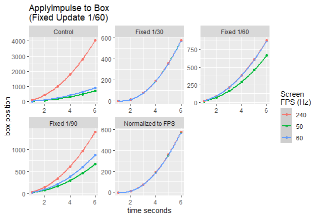
Overall, the fixed update method is effective but the selection of timestep is important as too high a time step may create differences in performance for players with lower screen fps relative to the selected timestep.
This results are encouraging and offer a couple of different methods to account for the screen fps to applyimpulse issue. However, a major limitation of this experiment is that it was done in a controlled environment where impulse is applied by the script and not by the player. In my original test of the normalized method within my game I still observed differences between different fps. This experiment confirms that the difference I observed was not due to issues in the method. Potentially, there is another issue when it comes to how user input is handled dependent upon screen fps. Perhaps when I apply the impulse in the 240 hz condition the impulse is applied sooner than that in the 60 Hz condition and this allows for the performance difference I see. I haven’t thought this all the way out yet but remember that reaction time video I posted previously? Maybe the differences he saw in his reaction time were more related to how well the machine detects the mouse click than the speed at which the screen changes color. At any rate this was a worthwhile exercise and hopefully it helps others who may run into this problem.
Supplemental material
All the code I used to create these graphs. Done in R
library(ggplot2)

data50=data.frame(t=c(1,2,3,4,5,6),p=c(21,80,178,311,484,696))
data60=data.frame(t=c(1,2,3,4,5,6),p=c(27,103,230,408,635,913))
data240=data.frame(t=c(1,2,3,4,5,6),p=c(105,436,996,1784,2803,4050))

dataall=rbind(data50,data60,data240)
dataall$Hz=rep(c('50','60','240'),each=6)

summary(lm(p~t+I(t^2),data50))
summary(lm(p~t+I(t^2),data60))
summary(lm(p~t+I(t^2),data240))
summary(lm(p~t*Hz+I(t^2)*Hz,dataall))

ggplot(dataall,aes(t,p,color=Hz))+
  geom_point()+
  geom_smooth(method = 'lm',formula = 'y~poly(x,2)')+
  xlab('time seconds')+
  ylab('box position')+
  labs(color="Screen\nFPS (Hz)")+
  ggtitle("ApplyImpulse to Box (Control)")

data50f=data.frame(t=c(1,2,3,4,5,6),p=c(-3,10,74,189,356,575))
data60f=data.frame(t=c(1,2,3,4,5,6),p=c(-3,10,74,189,355,573))
data240f=data.frame(t=c(1,2,3,4,5,6),p=c(-3,11,75,191,359,577))

dataallf=rbind(data50f,data60f,data240f)
dataallf$Hz=rep(c('50','60','240'),each=6)

summary(lm(p~t*Hz+I(t^2)*Hz,dataallf))

ggplot(dataallf,aes(t,p,color=Hz))+
  geom_point()+
  geom_smooth(method = 'lm',formula = 'y~poly(x,2)')+
  xlab('time seconds')+
  ylab('box position')+
  labs(color="Screen\nFPS (Hz)")+
  ggtitle("ApplyImpulse to Box\n(Normalize to 60 FPS)")

data50fi=data.frame(t=c(1,2,3,4,5,6),p=c(9,38,87,157,246,356))
data60fi=data.frame(t=c(1,2,3,4,5,6),p=c(9,37,86,155,244,353))
data240fi=data.frame(t=c(1,2,3,4,5,6),p=c(9,39,88,157,247,353))

dataallfi=rbind(data50f,data60f,data240f)
dataallfi$Hz=rep(c('50','60','240'),each=6)

summary(lm(p~t*Hz+I(t^2)*Hz,dataallfi))

ggplot(dataallfi,aes(t,p,color=Hz))+
  geom_point()+
  geom_smooth(method = 'lm',formula = 'y~poly(x,2)')+
  xlab('time seconds')+
  ylab('box position')+
  labs(color="Screen\nFPS (Hz)")+
  ggtitle("ApplyImpulse to Box\n(Fixed Update 1/30)")

data50fi6=data.frame(t=c(1,2,3,4,5,6),p=c(16,71,161,291,459,665))
data60fi6=data.frame(t=c(1,2,3,4,5,6),p=c(21,91,212,383,604,876))
data240fi6=data.frame(t=c(1,2,3,4,5,6),p=c(22,93,215,386,608,881))

dataallfi6=rbind(data50fi6,data60fi6,data240fi6)
dataallfi6$Hz=rep(c('50','60','240'),each=6)

summary(lm(p~t*Hz+I(t^2)*Hz,dataallfi6))

ggplot(dataallfi6,aes(t,p,color=Hz))+
  geom_point()+
  geom_smooth(method = 'lm',formula = 'y~poly(x,2)')+
  xlab('time seconds')+
  ylab('box position')+
  labs(color="Screen\nFPS (Hz)")+
  ggtitle("ApplyImpulse to Box\n(Fixed Update 1/60)")

data50fi9=data.frame(t=c(1,2,3,4,5,6),p=c(16,71,164,294,461,670))
data60fi9=data.frame(t=c(1,2,3,4,5,6),p=c(21,91,212,383,604,876))
data240fi9=data.frame(t=c(1,2,3,4,5,6),p=c(34,148,342,616,971,1405))

dataallfi9=rbind(data50fi9,data60fi9,data240fi9)
dataallfi9$Hz=rep(c('50','60','240'),each=6)

summary(lm(p~t*Hz+I(t^2)*Hz,dataallfi9))

ggplot(dataallfi9,aes(t,p,color=Hz))+
  geom_point()+
  geom_smooth(method = 'lm',formula = 'y~poly(x,2)')+
  xlab('time seconds')+
  ylab('box position')+
  labs(color="Screen\nFPS (Hz)")+
  ggtitle("ApplyImpulse to Box\n(Fixed Update 1/90)")

dataallm=rbind(dataall,dataallf,dataallfi,dataallfi6,dataallfi9)
dataallm$method=rep(c("Control","Normalized to FPS","Fixed 1/30","Fixed 1/60","Fixed 1/90"),each=18)

ggplot(dataallm,aes(t,p,color=Hz))+
  geom_point()+
  geom_smooth(method = 'lm',formula = 'y~poly(x,2)')+
  xlab('time seconds')+
  ylab('box position')+
  labs(color="Screen\nFPS (Hz)")+
  ggtitle("ApplyImpulse to Box\n(Fixed Update 1/60)")+
  facet_wrap(~method,scales = "free")

 I’ve updated the example.